5 Essential Excel Tips for Accountants (with Screenshots!)

If you’re starting out as an accountant or you just want to improve how you work with spreadsheets, we guarantee that learning these Excel skills will come in very handy. And what’s more it’ll take you less than 30 minutes to learn them!

1. Paste Special

Paste special has come to the rescue on many occasions. Have you ever hit Ctrl +Z and just got a load of errors values because there’s no reference?

Paste special gives you options to keep formatting, paste only values, and transpose values (horizontally or vertically).

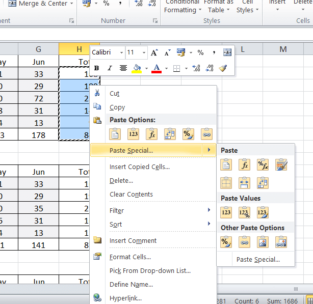
All you need to do is select the cells you want to copy, right click and then select paste special:

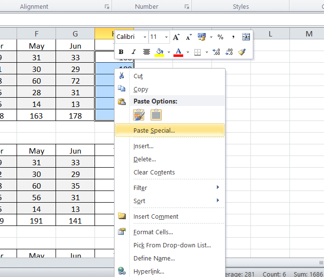
From there you’ll be able to choose what you do with the data: copying just values, formulas, formatting and various combinations to get your desired result.

2. Pivot Tables

Pivot tables are a really convenient way of sorting through a lot of data in a table, selecting only the columns you want to contrast and compare.

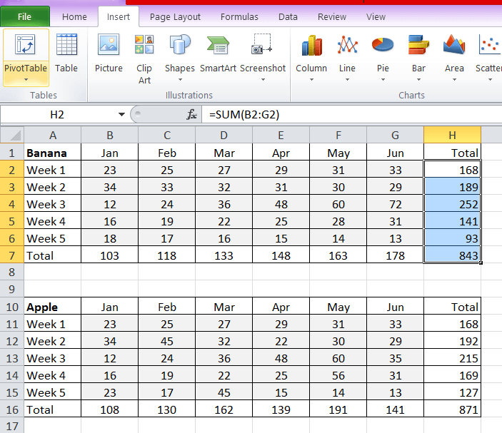
First put your data in a table (ctrl + T is a good shortcut) and then go to Insert > Pivot Table (top left, under File):

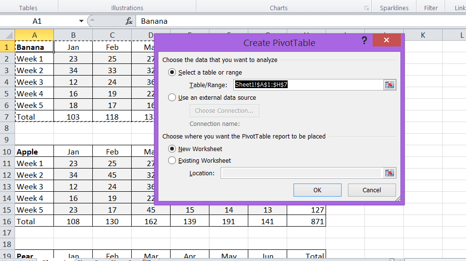
Then you can select the data you want to include (usually it gets selected automatically if you have one table formatted) and whether to create the table in a new worksheet or the existing one, then click ‘OK’:

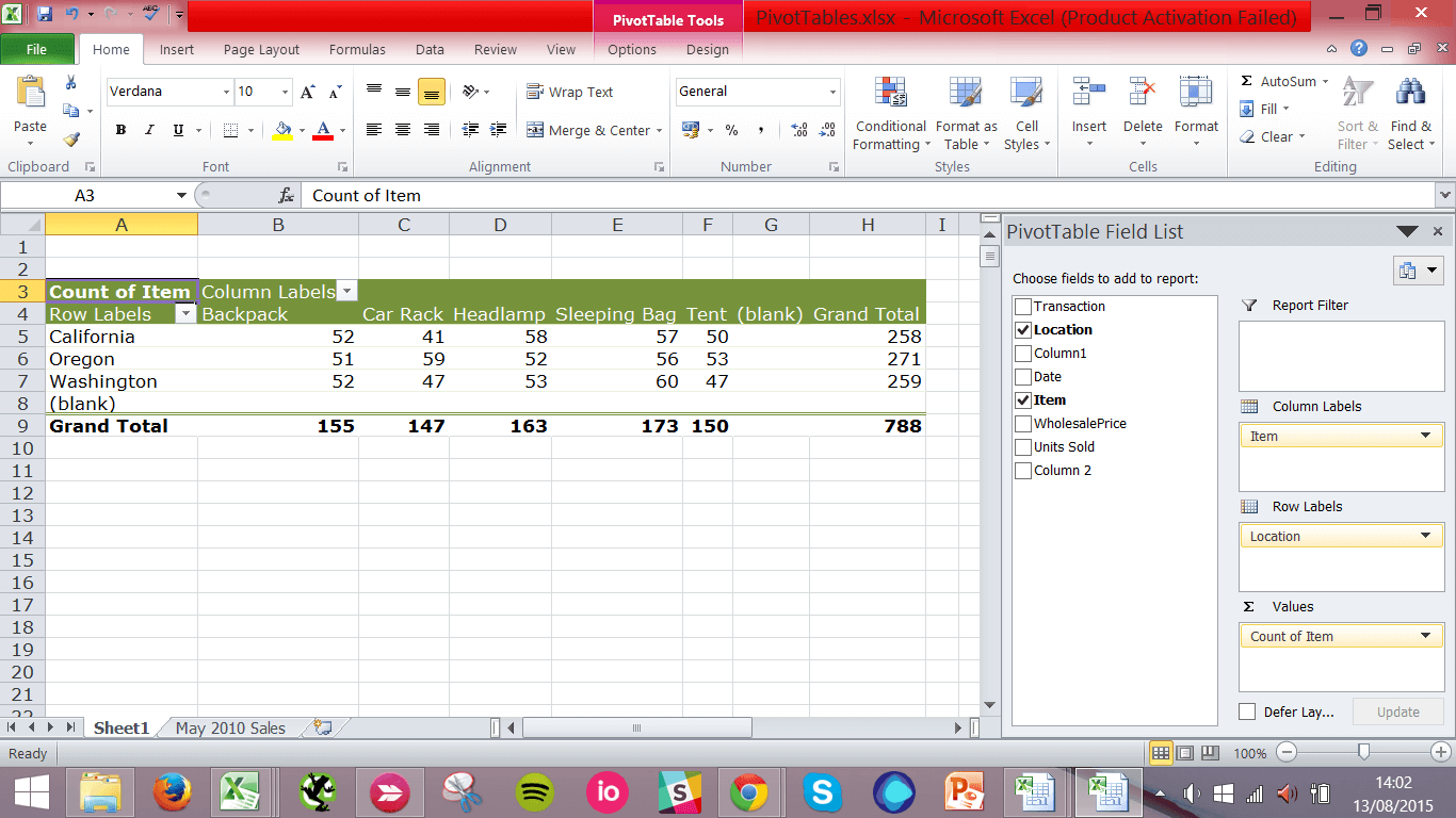
This is the example worksheet from Microsoft’s Pivot Table practice file:

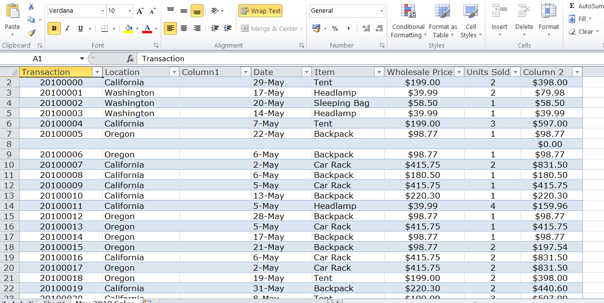
When we create a pivot table we can use the various columns from our original table as columns or headers in a new table, and use the count of item to do things like the below example: compare item sold with the location and how many times that item was sold. This is particularly useful when you have a list of transactions:

3. Copy Visible Cells Only

If you have hidden columns or rows in your document, this can be really useful as it prevents you from copying over unnecessary data.

Select the cells you want to copy as normal and then go to Home > Find & Select (top right) and click Go To Special:

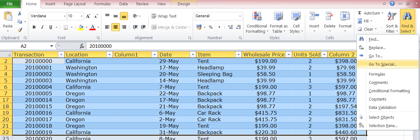
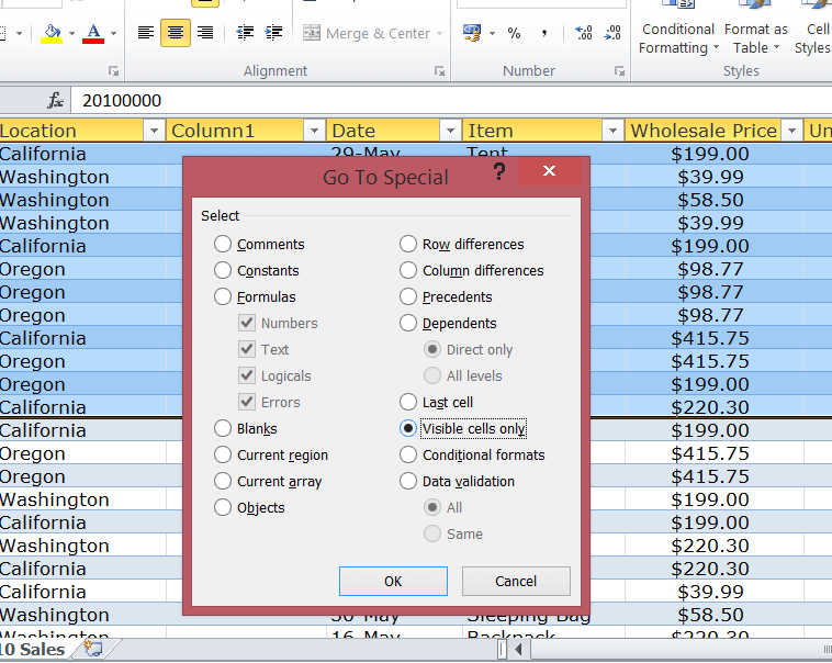
Then you can select copy only visible cells and hit ‘OK’.

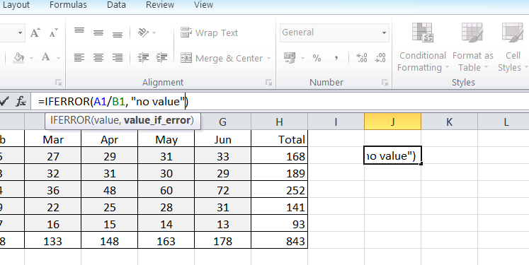
4. Fix #VALUE! Errors

This one isn’t that tricky to deal with: you just need to use an IFERROR command.

It’s useful when you’re dividing two values and there might be instances where a number is divided by, giving an error:

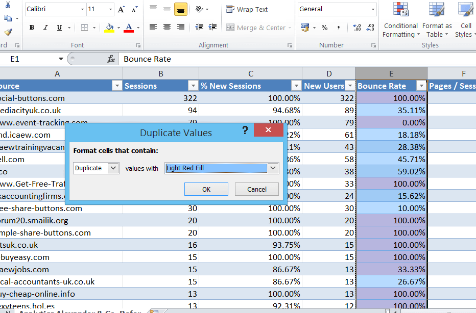
5. Highlight Duplicate Values

Select the data you want to check for duplicates then go to Home > Conditional Formatting > Highlight Cell Rules > Duplicate Values:

Click and you’ll be given formatting options to highlight the duplicate cells. We’ve chosen light red fill here:

We hope you’ve found this quick guide useful. If you have any recommendations for other quick Excel tips you’d like to see, get in touch with us on Twitter.